
The Art and Science of Feature Engineering in Machine Learning
A Comprehensive Guide for Both Beginners and Practitioners
1. Introduction to Feature Engineering
Feature engineering is both an art and science within the realm of machine learning, serving as the bridge between raw data and effective models. At its core, it involves transforming raw data into features that better represent the underlying patterns, enabling machine learning algorithms to perform more effectively. While modern deep learning approaches may attempt to automate some aspects of feature engineering, the process remains fundamentally important across virtually all data science applications.
Consider feature engineering as similar to how a chef prepares ingredients before cooking. Raw ingredients (data) must be cleaned, cut, measured, and sometimes pre-cooked (transformed) before they can be combined into a delicious meal (effective model). The quality of preparation directly influences the final dish, just as the quality of feature engineering directly impacts model performance.
Our Running Example: House Price Prediction
Throughout this article, we'll use house price prediction as our consistent example. Imagine we have a dataset containing information about houses, including:
- Numerical features: Square footage (1500 sq ft), number of bedrooms (3), number of bathrooms (2), lot size (0.25 acres)
- Categorical features: Neighborhood ("Greenwood"), house type ("Colonial"), heating system ("Forced air")
- DateTime features: Year built (1985), date of last renovation (2010-06-15)
- Text features: Property description ("Beautiful home with updated kitchen, hardwood floors, and large backyard")
Our goal is to predict the sale price of the house. We'll see how different feature engineering techniques can transform this raw data into more useful predictors.
2. The Machine Learning Pipeline
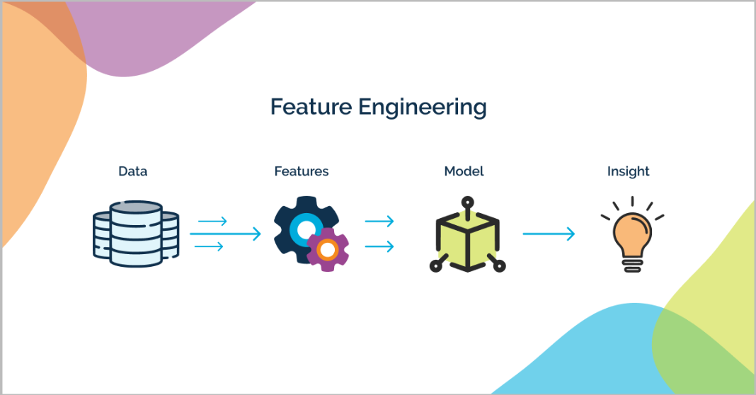
The machine learning pipeline consists of several crucial stages, with feature engineering occupying a central position. As illustrated in the diagram above, data typically flows from various sources through transformation processes before becoming useful for model training.
The process begins with raw data collection from multiple sources. This data is often messy, inconsistent, and not immediately suitable for machine learning algorithms. Next comes the data cleaning phase, where issues like missing values and outliers are addressed. Feature engineering follows, transforming and creating features that better represent the underlying patterns in the data.
After feature engineering, the prepared data is used for model training, followed by evaluation and fine-tuning. The insights derived from the model are then delivered to stakeholders for decision-making. This entire process is typically iterative, with feedback from later stages informing improvements in earlier stages.
House Price Prediction Pipeline
In our house price prediction example, the pipeline might look like:
- Data Collection: Gathering property records, including house attributes, location data, and historical sale prices
- Data Cleaning: Handling missing square footage values, correcting obvious data entry errors
- Feature Engineering: Converting neighborhood names to meaningful numerical representations, creating new features like "age of house," transforming skewed numerical features
- Model Training: Using the engineered features to train various regression models
- Evaluation: Testing the models on held-out data to measure prediction accuracy
- Deployment: Implementing the model in a real estate valuation system
3. Why Feature Engineering Matters
Feature engineering is a critical step in the machine learning pipeline for several compelling reasons. First and foremost, the quality of features directly impacts model performance. Well-engineered features can reveal hidden patterns that raw data obscures, enabling algorithms to learn more effectively with less data and computational resources.
Even the most sophisticated algorithms have limitations in their ability to automatically discover useful patterns. By crafting appropriate features, we effectively encode domain knowledge and human intuition into a form that algorithms can utilize. This process acts as a bridge between human understanding of the problem domain and the mathematical operations of learning algorithms.
As the seminal paper by Domingos (2012) noted, "feature engineering is the key factor that can make machine learning successful in practice." This observation remains valid today, even with advances in deep learning, which can sometimes reduce—but rarely eliminate—the need for feature engineering.
Impact on House Price Predictions
In our house price prediction scenario, consider these improvements through feature engineering:
- Raw data: A house built in 1985 and another built in 2020
- Engineered feature: House age (38 years vs. 3 years)
- Benefit: The model can now directly learn the relationship between age and depreciation/value, rather than having to infer complex patterns from seemingly arbitrary years
Similarly, instead of using raw square footage, we might create a "price per square foot" feature that normalizes house prices by size, making it easier for the model to identify whether a house is relatively expensive or inexpensive for its size.
Feature engineering can significantly reduce model complexity while improving performance. A simpler model with well-engineered features often outperforms complex models working with raw data. This leads to models that are more interpretable, computationally efficient, and easier to deploy and maintain in production environments.
4. Common Feature Engineering Techniques
Let's explore the most important feature engineering techniques, understanding not just how they work but why they're useful and when to apply them. For each technique, we'll continue with our house price prediction example to provide consistent context.
Real-world datasets often contain missing values, which most machine learning algorithms cannot handle directly. Missing data can occur due to collection errors, data corruption, or simply because some information was unavailable at the time of recording.
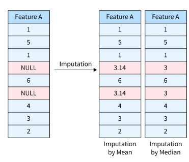
The simplest approach is to remove rows with missing values, but this can lead to significant data loss. A more sophisticated approach is imputation, where missing values are replaced with estimated values based on the available data.
Common imputation strategies include:
- Mean/Median/Mode Imputation: Replace missing values with the mean, median, or mode of the feature
- K-Nearest Neighbors Imputation: Estimate missing values based on similar data points
- Model-Based Imputation: Use machine learning models to predict missing values based on other features
import numpy as np
# Sample data with missing square footage
df = pd.DataFrame({'square_footage': [1500, 1800, np.nan, 2200]})
# Mean imputation
df['square_footage'].fillna(df['square_footage'].mean(), inplace=True)
House Price Example: Missing Square Footage
In our housing dataset, suppose we have missing values for the square footage of some properties. Since square footage is a critical feature for price prediction, we can't simply drop these rows. Instead, we might:
- Calculate the mean square footage for houses with the same number of bedrooms in the same neighborhood
- Use this mean value to fill in the missing values
- Consider adding a binary "was_imputed" feature to allow the model to account for the uncertainty in these values
This approach preserves our dataset size while providing reasonable estimates for the missing values.
Machine learning algorithms typically work with numerical data. However, real-world datasets often contain categorical variables like neighborhood names, house types, or heating system types. To make these usable for algorithms, we need to convert them to numerical formats through encoding techniques.
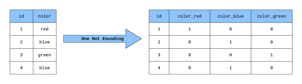
One-Hot Encoding

One-hot encoding creates binary columns for each category. Each of these columns contains 1 where the original value was present and 0 everywhere else. This approach is particularly useful when there's no ordinal relationship between categories.
df = pd.DataFrame({'house_type': ['Colonial', 'Ranch', 'Tudor', 'Colonial']})
# One-hot encoding
df_encoded = pd.get_dummies(df, columns=['house_type'])
Label Encoding
Label encoding replaces each category with a unique integer. This approach is more appropriate when there's an inherent order to the categories (like "low", "medium", "high").
# Sample data with ordinal property condition
df = pd.DataFrame({'condition': ['poor', 'fair', 'good', 'excellent']})
# Label encoding
le = LabelEncoder()
df['condition_encoded'] = le.fit_transform(df['condition'])
House Price Example: Encoding Neighborhoods and House Types
In our dataset:
- For neighborhoods (e.g., "Greenwood", "Riverside", "Downtown"), we'd use one-hot encoding since there's no inherent order to these values. This creates binary columns like "is_greenwood", "is_riverside", etc.
- For house condition ratings ("poor", "fair", "good", "excellent"), we'd use label encoding with values 0, 1, 2, 3 to preserve the ordinal relationship.
This allows our prediction model to properly understand and utilize these categorical features.
Feature scaling is essential when features have different units or ranges. Without scaling, features with larger values might dominate the learning process regardless of their actual importance. Scaling ensures all features contribute appropriately to the model.

Min-Max Scaling
Min-max scaling (normalization) transforms values to a specific range, typically [0,1]. This preserves the shape of the original distribution while constraining the range.
# Sample house data
df = pd.DataFrame({
'square_footage': [1500, 2500, 1800, 3000],
'price': [300000, 450000, 320000, 500000]
})
# Min-max scaling
scaler = MinMaxScaler()
df['square_footage_scaled'] = scaler.fit_transform(df[['square_footage']])
Standardization
Standardization (Z-score normalization) transforms the data to have a mean of 0 and a standard deviation of 1. This is particularly useful for algorithms like SVM, logistic regression, and neural networks.
# Standardization
scaler = StandardScaler()
df['square_footage_standardized'] = scaler.fit_transform(df[['square_footage']])
House Price Example: Scaling House Features
In our housing dataset, the features have widely different scales:
- Square footage: typically 1,000-5,000
- Number of bedrooms: typically 1-6
- Lot size: might be 0.1-2 acres
- Year built: values like 1950-2023
Without scaling, square footage and year built would dominate the model's learning process simply because their absolute values are much larger. By applying standardization, we transform these features to comparable scales, allowing the model to appropriately weigh their importance.
Log transformation is particularly useful for handling skewed data distributions. Many real-world features, like prices or areas, often follow a right-skewed distribution with a long tail. Log transformation can make these distributions more symmetric and closer to normal, which benefits many machine learning algorithms.
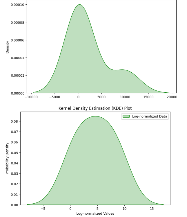
The transformation is simple: replace each value x with log(x) or log(x + 1) if x can be zero. The choice of log base (natural, base-10, etc.) doesn't typically matter much in practice, as it's just a constant scaling factor.
# Sample house price data (right-skewed)
df = pd.DataFrame({
'price': [250000, 320000, 285000, 950000, 1200000]
})
# Log transformation
df['price_log'] = np.log1p(df['price']) # log(x + 1) to handle zeros
House Price Example: Log Transforming Price Data
In our housing dataset, both the target variable (house prices) and some features like lot size tend to be right-skewed. For example:
- Most houses might be priced between $200,000-$500,000
- A smaller number of luxury homes might be priced at $1,000,000-$3,000,000
By applying log transformation to house prices, we create a more normally distributed target variable. This helps the model better learn the relationship between features and price, especially for those mid-range homes that make up the majority of the market. Models trained on log-transformed prices typically make more accurate predictions across the price spectrum.
Polynomial features allow linear models to capture non-linear relationships. They create new features by raising existing features to powers or creating interaction terms between different features. This technique can significantly increase model expressiveness without switching to more complex algorithms.
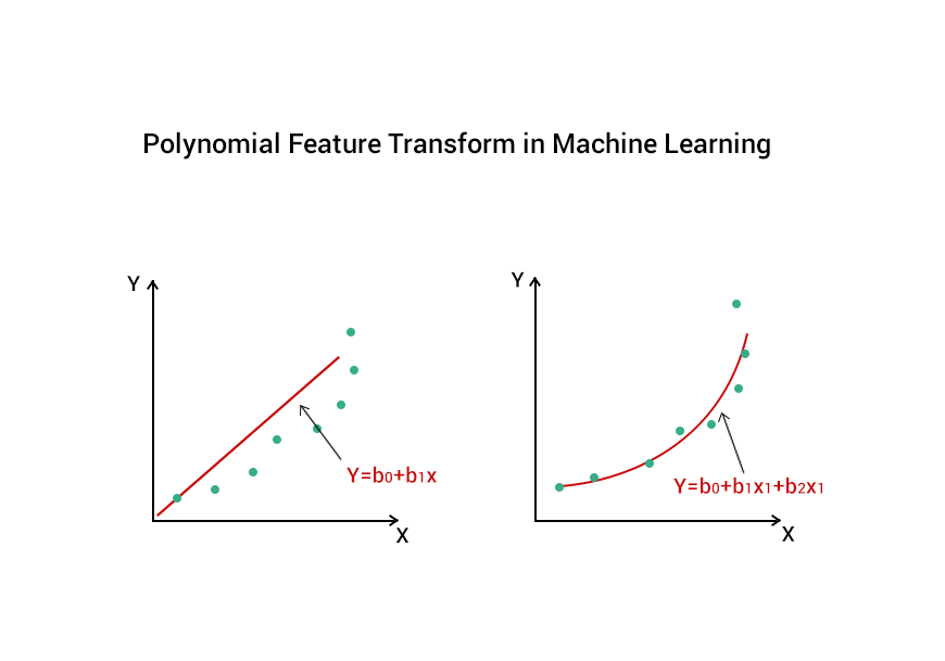
For example, if we have features X₁ and X₂, polynomial features of degree 2 would include X₁, X₂, X₁², X₂², and X₁X₂. This allows the model to capture quadratic relationships and interactions between variables.
# Sample housing data
df = pd.DataFrame({
'square_footage': [1500, 1800, 2200, 2500],
'lot_size': [0.2, 0.3, 0.25, 0.4]
})
# Generate polynomial and interaction features
poly = PolynomialFeatures(degree=2)
X_poly = poly.fit_transform(df[['square_footage', 'lot_size']])
# X_poly now contains original features, squared terms, and interactions
House Price Example: Creating Polynomial Features
In our house price prediction task, the relationship between square footage and price may not be perfectly linear. Larger homes may command incrementally higher prices per square foot due to luxury status.
By creating a squared term for square footage, our model can capture this non-linear relationship. Similarly, the interaction between lot size and square footage might be important - a large house on a small lot might be less valuable than the same house on a spacious lot.
Creating polynomial features would generate:
- square_footage² - captures the non-linear effect of home size
- lot_size² - captures the non-linear effect of land
- square_footage × lot_size - captures how these features interact
These new features enable even a simple linear regression model to capture complex relationships in the data.
Binning (or discretization) transforms continuous numerical variables into categorical bins. This technique can help capture non-linear relationships and make the model more robust to outliers and noise. It's especially useful when there are distinct thresholds in the relationship between a feature and the target.

Binning can be performed with equal-width bins, equal-frequency bins, or custom bins based on domain knowledge.
df = pd.DataFrame({
'house_age': [2, 5, 12, 25, 40, 60, 75]
})
# Custom binning with meaningful labels
bins = [0, 5, 20, 50, np.inf]
labels = ['new', 'recent', 'established', 'historic']
df['age_category'] = pd.cut(df['house_age'], bins=bins, labels=labels)
House Price Example: Binning House Age
In our housing dataset, the effect of a house's age on its price isn't strictly linear. There might be different market dynamics for:
- New construction (0-5 years): Premium prices for modern designs and new systems
- Recent homes (6-20 years): Slightly depreciated but still modern
- Established homes (21-50 years): May need some updates, priced lower
- Historic homes (51+ years): May have historical value or charm, possibly commanding higher prices again
By binning the continuous "house age" variable into these categories, we allow our model to learn different pricing effects for each age group, capturing the non-linear relationship between age and value.
Date and time variables contain rich information that can be extremely valuable for predictions. However, in their raw form (e.g., "2023-05-15"), they're not directly usable by most algorithms. Transforming dates into meaningful numerical components unlocks their predictive power.

Common date-time features include year, month, day, day of week, quarter, is_weekend, is_holiday, etc. The specific features to extract depend on the domain and the patterns you expect to find in the data.
df = pd.DataFrame({
'sale_date': ['2022-06-15', '2022-12-03', '2023-01-20', '2023-05-07']
})
# Convert to datetime and extract features
df['sale_date'] = pd.to_datetime(df['sale_date'])
df['sale_year'] = df['sale_date'].dt.year
df['sale_month'] = df['sale_date'].dt.month
df['sale_quarter'] = df['sale_date'].dt.quarter
df['is_spring_summer'] = df['sale_month'].isin([3, 4, 5, 6, 7, 8]).astype(int)
House Price Example: Seasonal Housing Market Patterns
In our housing dataset, both the build date and sale date contain valuable information. From these dates, we can extract:
- House age: Current year - build year (a more relevant feature than the raw build year)
- Sale season: Spring/summer sales often command higher prices than winter sales
- Year of sale: Captures market trends over time
- Month of sale: Captures seasonal patterns
For instance, a house that sold in June 2022 might have achieved a higher price than an identical house sold in January 2022 due to the higher demand during summer months. These seasonal patterns can be captured through proper datetime feature engineering.
Text data presents unique challenges for machine learning, as it's inherently unstructured. Feature engineering for text involves converting text into numerical representations that capture semantic meaning while being usable by algorithms.
Common approaches include:
- Bag of Words: Counts word occurrences, ignoring order
- TF-IDF: Weighs words by their frequency in the document and inverse frequency across all documents
- Word Embeddings: Maps words to dense vectors that capture semantic relationships
# Sample house descriptions
descriptions = [
"Beautiful home with updated kitchen and hardwood floors",
"Spacious house with large backyard and pool",
"Charming cottage near downtown with original features"
]
# Convert to TF-IDF features
vectorizer = TfidfVectorizer(max_features=50)
X_tfidf = vectorizer.fit_transform(descriptions)
# X_tfidf now contains numerical features representing the text
House Price Example: Extracting Value from Property Descriptions
Property listings often include descriptive text that contains valuable information not captured in structured fields. For our house with the description "Beautiful home with updated kitchen, hardwood floors, and large backyard":
Using TF-IDF vectorization, we can convert this text into features that highlight distinctive terms. Words like "updated," "hardwood," and "large" might be assigned higher weights if they appear relatively infrequently in the overall dataset. The model can then learn that properties described with these terms tend to command higher prices.
Additionally, we might extract specific high-value keywords from descriptions:
- has_updated_kitchen: 1 (detected "updated kitchen")
- has_hardwood_floors: 1 (detected "hardwood floors")
- has_large_yard: 1 (detected "large backyard")
These binary features can provide significant predictive power alongside the numerical and categorical features.
5. Advanced Feature Engineering Techniques
Beyond the common techniques we've discussed, there are advanced approaches that can further enhance model performance. These methods often require deeper domain knowledge or more sophisticated implementation but can provide substantial benefits for complex problems.
Feature Extraction with Principal Component Analysis (PCA)
PCA reduces the dimensionality of data while preserving as much variance as possible. It creates new features (principal components) that are linear combinations of the original features, ordered by the amount of variance they explain.
# Apply PCA to housing features
pca = PCA(n_components=2)
housing_features = df[['square_footage', 'bedrooms', 'bathrooms', 'lot_size']]
components = pca.fit_transform(housing_features)
df['pc1'] = components[:, 0]
df['pc2'] = components[:, 1]
House Price Example: Using PCA for Size Index
In our housing dataset, several features relate to the overall size of a property: square footage, number of bedrooms, number of bathrooms, and lot size. These features are often correlated.
By applying PCA, we might find that the first principal component effectively represents an overall "size index" that combines these features optimally. This can reduce multicollinearity in our model while still capturing the important size-related variance that influences price.
Clustering as a Feature
Clustering algorithms can group similar data points and provide cluster assignments as new features. This can help models identify patterns based on these natural groupings.
# Create cluster features
kmeans = KMeans(n_clusters=4, random_state=0)
location_features = df[['latitude', 'longitude']]
df['location_cluster'] = kmeans.fit_predict(location_features)
House Price Example: Neighborhood Clustering
Instead of relying solely on predefined neighborhood boundaries, we could use the geographical coordinates (latitude and longitude) of houses to identify natural clusters. These clusters might represent micro-neighborhoods that aren't captured in official designations but have distinct pricing characteristics.
For example, houses within walking distance to a popular park or school might form a cluster with higher values, even if they technically span multiple official neighborhoods. The cluster assignment becomes a powerful feature that captures this implicit location premium.
Feature Generation with Domain Knowledge
Perhaps the most powerful form of feature engineering comes from domain expertise. Subject matter experts can identify meaningful combinations or transformations of raw data that capture important relationships.
House Price Example: Real Estate Domain Features
A real estate expert might suggest features like:
- Price per square foot: house_price / square_footage
- Bedroom-to-bathroom ratio: bedrooms / bathrooms
- Land-to-building ratio: lot_size / square_footage
- Renovation recency: current_year - last_renovation_year
- School quality index: weighted combination of nearby school ratings
These domain-specific features often capture important aspects of property valuation that might not be apparent from raw data alone.
Time-Series Feature Engineering
For data with temporal components, specialized time-series features can be extremely valuable:
- Lagged Features: Including previous values of a variable
- Rolling Statistics: Moving averages, standard deviations, etc.
- Growth Rates: Percentage changes over various time periods
- Seasonal Components: Extracted through decomposition methods
House Price Example: Market Trend Features
If our dataset spans multiple years, we might create features that capture market trends:
- 3-month price trend: Average price change in the neighborhood over the last 3 months
- Seasonal price index: How much prices typically change in the current month based on historical patterns
- Days-on-market trend: Whether houses are selling faster or slower than in previous months
These temporal features can help the model account for market dynamics when predicting house prices.
6. Best Practices and Common Pitfalls
Feature engineering is as much an art as it is a science. Here are some best practices to maximize its effectiveness and pitfalls to avoid:
Best Practices
Understand the Domain
The most powerful feature engineering comes from deep understanding of the problem domain. Consult with subject matter experts to identify meaningful features that might not be obvious from the data alone. In our housing example, speaking with real estate agents might reveal that homes within a 5-minute walk of public transit command a significant premium - a feature you wouldn't create without this domain knowledge.
Start Simple, Then Iterate
Begin with basic transformations and gradually add complexity as needed. This methodical approach helps identify which feature engineering techniques actually improve model performance. For our house price model, we might start with simple scaling and encoding, establish a baseline, and then progressively add polynomial features, interaction terms, and domain-specific features while measuring the impact on performance.
Use Cross-Validation for Evaluation
Evaluate the impact of feature engineering using proper cross-validation to avoid overfitting to the peculiarities of a single train-test split. This helps ensure that the engineered features genuinely improve model generalization. For our housing dataset, we might use 5-fold cross-validation to reliably assess whether log-transforming price or adding polynomial features actually improves prediction accuracy.
Document Your Transformations
Maintain clear documentation of all feature transformations for reproducibility and future reference. This is especially important for complex pipelines. For our house price model, we would document the exact binning thresholds for house age, the specific method used for imputing missing square footage values, and any other transformations applied.
Common Pitfalls
Data Leakage
One of the most serious pitfalls is data leakage, where information from outside the training data (including from the target variable) improperly influences feature creation. For example, if we impute missing values using statistics calculated on the entire dataset (including the test set), we're inadvertently leaking information. Always perform feature engineering within the cross-validation framework, applying transformations separately to each training fold.
House Price Example: Avoiding Leakage
A leakage error in our housing dataset might be encoding the neighborhood categories based on average house prices, effectively leaking the target variable into the features. Instead, we should use one-hot encoding or other methods that don't incorporate price information.
Overly Complex Features
Creating extremely complex features without theoretical justification can lead to overfitting. The model might learn patterns specific to the training data that don't generalize well. Prefer interpretable features that have a clear relationship with the target variable.
House Price Example: Appropriate Complexity
Creating a 5th-degree polynomial for square footage would likely be excessive and lead to overfitting. A quadratic (2nd-degree) term may be sufficient to capture the non-linear relationship between home size and price.
Ignoring Feature Selection
Aggressive feature engineering can lead to a high-dimensional feature space, increasing the risk of overfitting. Consider feature selection techniques to identify and keep only the most informative features.
# Select top 10 features
selector = SelectKBest(f_regression, k=10)
X_selected = selector.fit_transform(X, y)
Not Handling Feature Engineering in Production
After deploying a model, it's crucial to apply the exact same feature engineering to new data. This requires implementing a reproducible feature engineering pipeline that can be applied consistently in production environments.
from sklearn.preprocessing import StandardScaler
from sklearn.impute import SimpleImputer
from sklearn.linear_model import LinearRegression
# Create a pipeline for reproducible transformations
pipeline = Pipeline([
('imputer', SimpleImputer(strategy='mean')),
('scaler', StandardScaler()),
('model', LinearRegression())
])
7. Conclusion
Feature engineering remains one of the most crucial aspects of effective machine learning, often making the difference between mediocre and exceptional model performance. By thoughtfully transforming raw data into informative features, we enable algorithms to better capture the underlying patterns and relationships relevant to the prediction task.
Throughout this comprehensive guide, we've explored numerous feature engineering techniques—from basic approaches like handling missing values and encoding categorical variables to more advanced methods like polynomial features and domain-specific transformations. Using our consistent house price prediction example, we've seen how each technique can be applied in a real-world context to improve model performance.
The key takeaways from this exploration include:
- Feature engineering is both an art and a science, requiring domain knowledge, creativity, and empirical validation
- Different techniques are appropriate for different types of data and modeling scenarios
- A methodical approach—starting with simple transformations and progressively adding complexity—often yields the best results
- Proper evaluation and documentation are essential to build reliable, reproducible models
As machine learning continues to evolve, feature engineering remains a critical skill for data scientists and machine learning engineers. While automated feature engineering tools are emerging, the most effective approaches still combine algorithmic techniques with human insight and domain expertise.
Whether you're predicting house prices, customer churn, stock movements, or any other target variable, investing time in thoughtful feature engineering will almost always pay dividends in improved model performance and more robust real-world applications.
Final Thoughts on Our House Price Example
Our house price prediction journey showcases the transformative power of feature engineering. Starting with raw data about house attributes, we've engineered numerous informative features:
- Transformed skewed price data with logarithms
- Created meaningful categories for house age through binning
- Extracted seasonal patterns from sale dates
- Developed domain-specific features like price-per-square-foot
These engineered features enable our model to capture the complex factors that influence house prices, resulting in more accurate predictions across diverse properties and market conditions. The same principles and techniques can be applied across virtually any machine learning domain to enhance model performance.
References and Further Reading
- Domingos, P. (2012). A few useful things to know about machine learning. Communications of the ACM, 55(10), 78-87.
- Zheng, A., & Casari, A. (2018). Feature engineering for machine learning: principles and techniques for data scientists. O'Reilly Media.
- Kuhn, M., & Johnson, K. (2019). Feature engineering and selection: A practical approach for predictive models. CRC Press.
- Guyon, I., & Elisseeff, A. (2003). An introduction to variable and feature selection. Journal of machine learning research, 3(Mar), 1157-1182.
إرسال تعليق